[ML] Back propagation

L : Total number of layers in network.
s(l) : number of units (bias unit not included) in layer (l)
K : number of out put unit.

For binary classification,

y = 0 or 1

there will be only 1 output unit, either 0 or 1

i.e:

h(x) ∈ R

----
For multi-class classification (K classes),
y ∈ R^(K)

K output units.

i.e:
h(x) ∈ R^(K)

------

Cost function:

-------
Now, let's minimize the cost function output.

Backpropagation algorithm:

δj^(l) = "error of node (j) in layer (l).

With the use of matrix, we can get rid of j, only keep the layer (l).

i.e:
δ^l = a^l - y , each symbol as a matrix of   dimention (K X 1)

So, if we want layer 4 error δ,

δ^4 = a^4 - y for each node K.

δ^3 = (⊖^3)[transpose]δ^4 .* g'(z^3)

Steps:

1. Forward propagation to get the last layer L's  [a] nodes results
2. Use the last layer [a] result to calculate the last layer's  δ value.
3. There's no δ^1, layer 1 is the input layer, no errors.
4. Use ∆^l as accumulative results of all the δ^l of every training examples.
i.e:
    a^l * δ^(l+1)
5. vectorize it.

i.e:
a^l is 5 X 1 matrix, that is, for that layer l, have 5 nodes.
δ^(l+1) is 1 X 4 matrix, that is, for last layer, has only 4 nodes, K = 4.

a^l * δ^(l+1) is a 5 X 4 matrix.

Every a(i) nodes times the δ1 forms a column of 5 X 1 matrix. And
there are 4 δ.

---------------
Forward propagation:

[a] is called activation function, i.e g(h(x))

Steps by steps:

Simplified explaination:

-------------

Back propagate, consider each layer has only 1 node.

i.e , to calculate δ2^(2), from right to left, we have ⊖(12)^2 * δ1^(3) + ⊖(22)^2 * δ2^(3)

When we say :
 ⊖(12) , means that 1 is for node 1, 2 is for the 2nd feature.

----------------
Implementation detail:

Reshape command:
By unrolling, same as for loop unrolling, make all elements into a row vector.

While need the original vector, reshape from the unrolled row vector.


e.g:
octave:

theta1 = ones(10,11)
theta2 = 2*ones(10,11)
theta3 = 3*ones(1,11)

% unroll
thetaVec = [ theta1(:); theta2(:); theta3(:)];

reshape(thetaVec(1,110),  10, 11) % arg1: input vector;  arg2: row count; arg3: col count

symbol meaning:
***  X12 , ALWAYS, which NODE, which FEATURE.  i.e : Node 1, Feature 2.


------------------
Gradient checking:

Numerical estimation of gradients:
Simple, use J(x +/- ε) to find the 2 points slope, that could estimate the J(x).
Use 2 sides approach than 1 side approach, which former is more accurate.
(free from error causes, which average will cover that.)

i.e:

While  ⊖ is in n dimention:
 ⊖ ∈ R^n  ( ⊖ is unroll with ⊖1, ⊖2, ..., ⊖n features)

So, after compute the approximate value of deferentiated value, compare

with the backpropagation result, they should be close, otherwise, our backpropagation

code should have a bug...

steps:

----------------

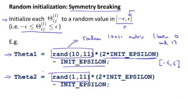
Random initialization:

We need initial value for ⊖.  

Don't do zero initialization for all the ⊖.

It's meaning less...

Thus, using random value for every ⊖.

--------------
 So, let's start using this:

Pick a network architecture(connectivity pattern between neurons)
 (number of nodes in hidden layers, default is that each hidden layer has same nodes,
 the more hidden layers the better.)
 (number of input nodes, i.e features)
 (number of output nodes, i.e number of classes, i.e
 y=
 [1
 ...
 0] ;
 [0
  1
  ...
  0];
 [0
  0
  1
  ...
  0];
 
 

 
------------------

Training a neural network:

Beware that since this is a classification problem, the cost function is non-convex,
i.e, could stuck in local minimum.
However, in practice, this isn't a issue due to even it's local minimum, it's good enough
for the h(x) to predict future input.

graph e.g:

-----------------